Overview of Artificial Intelligence

What artificial intelligence means

Artificial intelligence (AI) is a branch of computer science concerned with using computers to simulate human ways of thinking and acting, so that machines can take over certain kinds of work that would otherwise rely on people.

The structure of the AI field

The discipline of AI covers several connected areas:

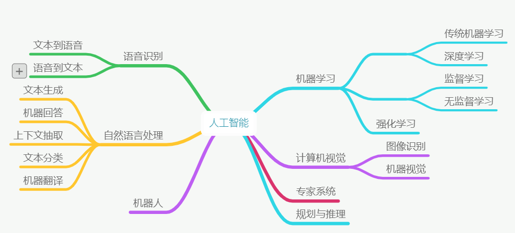
• Machine Learning: a subfield of AI that studies core algorithms, principles, and methods. Many other AI areas rely on what machine learning provides.
• Computer Vision: technologies that enable computers to process, recognize, and understand images and video.
• Natural Language Processing: technologies for understanding human language.
• Speech Processing: technologies for recognizing, understanding, and synthesizing speech.

How AI differs from traditional software

• Traditional software follows instructions and ideas already provided by humans. The solution is known before execution, so the program cannot go beyond human understanding built into it.
• Artificial intelligence tries to move past those fixed boundaries by allowing computers to acquire new capabilities through learning, making it possible to tackle problems that are difficult for conventional software.

Course scope and learning characteristics

What the course includes

Why the subject feels difficult

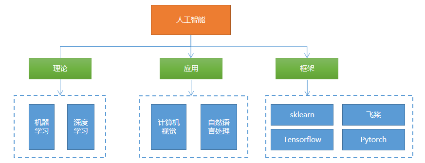
This area is broad and demanding:

• It spans machine learning, deep learning, computer vision, NLP, and commonly used frameworks.
• It is hard at every stage: getting started is difficult, improving is difficult, and applying what you learn is also difficult.
• Some mathematical background is needed, whether that means remembering conclusions, calling APIs correctly, analyzing formulas, or deriving them.
• Repetition is essential:
• first pass: understand the main ideas,
• second pass: grasp the core concepts,
• third pass: become familiar with coding,
• fourth pass: deepen understanding and learn to apply it.
• The more you study, the deeper it gets.

A practical way to study

A sensible learning path is:

• understand first, focus on meaning before details;
• move from easy to hard, listen before writing, go from rough understanding to fine understanding;
• skip points that are too difficult at the moment and focus on the big picture;
• read materials from different authors and learn from different instructors.

Core ideas in machine learning

What machine learning is

Herbert Simon, a scholar who received the Turing Award in 1975 and the Nobel Memorial Prize in Economic Sciences in 1978, gave a broad definition of learning: if a system can improve its performance by carrying out some process, then that process is learning. In other words, the purpose of learning is performance improvement.

Tom Mitchell, a professor of machine learning and artificial intelligence at Carnegie Mellon University, gave a more operational definition in his classic textbook Machine Learning: for some task T and some performance measure P, if a computer program improves its performance on T, as measured by P, through experience E, then the program is said to have learned from E.

A simple analogy is basketball shooting practice:

• Task (T): taking shots
• Performance (P): shooting accuracy
• Experience (E): repeated practice

As practice accumulates and accuracy improves, learning has taken place.

Why machine learning is needed

Machine learning matters for at least three reasons:

1. it allows programs to improve themselves;
2. it helps solve problems whose algorithms are too complex, or for which no known algorithm exists;
3. the learning process can also help humans gain insight into the things being studied.

The formal view of machine learning

Modeling

In a simplified formal sense, machine learning can be seen as using statistics and inference on data to find a function that maps an input X to an expected output Y:

$ Y = f(x)$

That function, together with the parameters that determine it, is called a model.

Evaluation

Even when the input is known, the function’s output—the prediction—usually differs somewhat from the real output—the target. Because of this, an evaluation system is needed to measure the error and judge how good or bad the function is.

Optimization

Learning is fundamentally about improving performance. By repeatedly refining an algorithm through data, the model’s predictive accuracy is continuously improved until it reaches a solution that is good enough for practical needs. That refinement process is machine learning.

Main categories of machine learning

Supervised, unsupervised, semi-supervised, and reinforcement learning

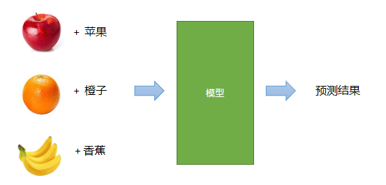
Supervised learning

When the outputs of training data are known in advance—that is, the data is labeled—the model can be trained and adjusted against those known outputs. This is supervised learning.

Unsupervised learning

When outputs are unknown, the system relies only on relationships within the input data in order to divide it into groups or categories. This is unsupervised learning.

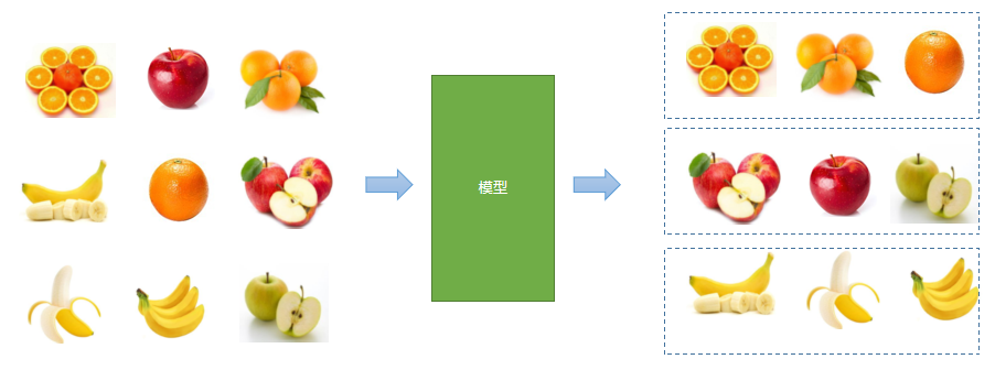
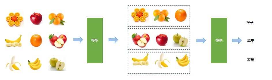
Semi-supervised learning

A common hybrid approach is to first group data using unsupervised learning, then manually label some of it and use supervised learning to predict outputs. For example, similar fruits may first be clustered, and then their categories identified.

Reinforcement learning

In reinforcement learning, the system is guided by rewards and penalties tied to different decisions. After enough training, it becomes more and more likely to produce actions closer to the desired result.

Batch learning and incremental learning

Batch learning

In batch learning, training and application are separate. A model is trained on the full training dataset first, then used for prediction in real-world use. If the results are not good enough, training is done again, and the cycle repeats.

Incremental learning

In incremental learning, training and application happen together. The model learns new information in small additions while it is already being used—training while predicting.

Model-based learning and instance-based learning

Model-based learning

This approach builds a mathematical model from sample data to describe the relationship between input and output. New inputs are then fed into that model for prediction.

For example:

<table> <thead> <tr> <th>Input (x)</th> <th>Output (y)</th> </tr> </thead> <tbody> <tr> <td>1</td> <td>2</td> </tr> <tr> <td>2</td> <td>4</td> </tr> <tr> <td>3</td> <td>6</td> </tr> <tr> <td>4</td> <td>8</td> </tr> </tbody> </table>

From these samples, the model is:

$y = 2x$

Prediction: when the input is 9, what is the output?

Instance-based learning

This approach does not build an explicit general formula first. Instead, it looks for past samples most similar to the input that needs prediction, and uses their outputs as the basis for an answer.

Example data:

<table> <thead> <tr> <th>Education (x1)</th> <th>Work Experience (x2)</th> <th>Gender (x3)</th> <th>Monthly Salary (y)</th> </tr> </thead> <tbody> <tr> <td>Bachelor</td> <td>3</td> <td>Male</td> <td>8000</td> </tr> <tr> <td>Master</td> <td>2</td> <td>Female</td> <td>10000</td> </tr> <tr> <td>PhD</td> <td>2</td> <td>Male</td> <td>15000</td> </tr> </tbody> </table>

Prediction: Bachelor, 3, Male ==> salary?

The usual machine learning workflow

The standard process typically looks like this:

1. Data collection: manually collected data, automatic device collection, web crawling, and similar methods.
2. Data cleaning: remove nonstandard data, data with large errors, and meaningless data.

The first two steps belong to data handling, which also includes things like data retrieval, data mining, and crawling.

1. Choose a model or algorithm.
2. Train the model.
3. Evaluate the model.
4. Test the model.

Steps 3 through 6 form the core machine learning process, involving algorithms, frameworks, tools, and related techniques.

1. Apply the model.
2. Maintain the model.

Typical applications of machine learning

Representative use cases include:

1. stock price prediction;
2. recommendation engines;
3. natural language processing;
4. speech tasks such as speech recognition and speech synthesis;
5. image recognition and face recognition;
6. and many others.

Fundamental problem types in machine learning

Regression

Regression means finding a model from known input-output pairs and using it to predict an continuous output for unseen inputs.

Examples include:

• predicting housing prices from area, location, construction year, and other factors;
• predicting a stock price from external conditions;
• forecasting crop yield from agricultural and weather data;
• calculating the similarity between two faces.

Classification

Classification means finding a model from known input-output pairs and using it to predict a discrete output.

Examples include:

• handwritten digit recognition, which is a 10-class classification problem;
• recognizing fruits, flowers, or animals;
• industrial defect inspection, such as good product vs defective product, a binary classification task;
• identifying the sentiment expressed by a sentence: positive, negative, or neutral.

Clustering

Clustering groups inputs according to similarity, without relying on known labels.

Examples include:

• deciding which wheat grains belong to the same variety based on grain data;
• determining which customers are interested in a certain product based on browsing and purchase history on an e-commerce site;
• identifying customers with higher similarity to one another.

Dimensionality reduction

Dimensionality reduction aims to lower data complexity or reduce data size while keeping performance loss as small as possible.

Course content summary

Data preprocessing

Why preprocessing matters

Data preprocessing mainly serves three purposes:

1. remove invalid, nonstandard, and incorrect data;
2. fill in missing values;
3. unify ranges, units, formats, and data types so later computation becomes easier.

Common preprocessing methods

Standardization (mean removal)

Standardization transforms each column of the sample matrix so that its mean becomes 0 and its standard deviation becomes 1.

Given three numbers a, b, and c, their mean is:

$$ m = (a + b + c) / 3 \ a’ = a - m \ b’ = b - m \ c’ = c - m $$

After mean removal, the new average is 0:

$$ (a’ + b’ + c’) / 3 =((a + b + c) - 3m) / 3 = 0 $$

The post-processing standard deviation is:

$s = sqrt(((a - m)^2 + (b - m)^2 + (c - m)^2)/3)$

$a’’ = a / s$

$b’’ = b / s$

$c’’ = c / s$

$$s’’ = sqrt(((a’ / s)^2 + (b’ / s) ^ 2 + (c’ / s) ^ 2) / 3) $$

$=sqrt((a’ ^ 2 + b’ ^ 2 + c’ ^ 2) / (3 *s ^2))$

$=1$

The standard deviation, often written as σ, is the square root of the arithmetic mean of squared deviations from the mean. It reflects how dispersed a dataset is.

Code example:

<table> <thead> <tr> <th>1 2 3 4 5 6 7 8 9 10 11 12 13 14 15 16 17 18 19 20 21 22 23 24</th> <th># 数据预处理之：均值移除示例 import numpy as np import sklearn.preprocessing as sp # 样本数据 raw_samples = np.array([ [3.0, -1.0, 2.0], [0.0, 4.0, 3.0], [1.0, -4.0, 2.0] ]) print(raw_samples) print(raw_samples.mean(axis=0)) # 求每列的平均值 print(raw_samples.std(axis=0)) # 求每列标准差 std_samples = raw_samples.copy() # 复制样本数据 for col in std_samples.T: # 遍历每列 col_mean = col.mean() # 计算平均数 col_std = col.std() # 求标准差 col -= col_mean # 减平均值 col /= col_std # 除标准差 print(std_samples) print(std_samples.mean(axis=0)) print(std_samples.std(axis=0))</th> </tr> </thead> <tbody> <tr> <td></td> <td></td> </tr> </tbody> </table>

The same result can also be obtained with sp.scale from sklearn:

<table> <thead> <tr> <th>1 2 3 4</th> <th>std_samples = sp.scale(raw_samples) # 求标准移除 print(std_samples) print(std_samples.mean(axis=0)) print(std_samples.std(axis=0))</th> </tr> </thead> <tbody> <tr> <td></td> <td></td> </tr> </tbody> </table>

Min-max scaling

This method rescales each column in the sample matrix so that the minimum and maximum fall into the same fixed interval.

Suppose b is the minimum and c is the maximum among a, b, and c:

$$ a’ = a - b $$

$$ b’ = b - b $$

$$ c’ = c - b $$

The scaling is then:

$$ a’’ = a’ / c’ $$

$$ b’’ = b’ / c’ $$

$$ c’’ = c’ / c’ $$

After scaling, the minimum becomes 0 and the maximum becomes 1.

Example:

<table> <thead> <tr> <th>1 2 3 4 5 6 7 8 9 10 11 12 13 14 15 16 17 18 19</th> <th># 数据预处理之：范围缩放 import numpy as np import sklearn.preprocessing as sp # 样本数据 raw_samples = np.array([ [1.0, 2.0, 3.0], [4.0, 5.0, 6.0], [7.0, 8.0, 9.0]]).astype("float64") # print(raw_samples) mms_samples = raw_samples.copy() # 复制样本数据 for col in mms_samples.T: col_min = col.min() col_max = col.max() col -= col_min col /= (col_max - col_min) print(mms_samples)</th> </tr> </thead> <tbody> <tr> <td></td> <td></td> </tr> </tbody> </table>

The same operation can be done with a sklearn object:

<table> <thead> <tr> <th>1 2 3 4 5</th> <th># 根据给定范围创建一个范围缩放器对象 mms = sp.MinMaxScaler(feature_range=(0, 1))# 定义对象(修改范围观察现象) # 使用范围缩放器实现特征值范围缩放 mms_samples = mms.fit_transform(raw_samples) # 缩放 print(mms_samples)</th> </tr> </thead> <tbody> <tr> <td></td> <td></td> </tr> </tbody> </table>

Execution result:

<table> <thead> <tr> <th>1 2 3 4 5 6</th> <th>[[0. 0. 0. ] [0.5 0.5 0.5] [1. 1. 1. ]] [[0. 0. 0. ] [0.5 0.5 0.5] [1. 1. 1. ]]</th> </tr> </thead> <tbody> <tr> <td></td> <td></td> </tr> </tbody> </table>

Normalization

Normalization reflects proportions within each sample. Each feature value in a sample is divided by the sum of the absolute values of all features in that same sample. After transformation, the sum of absolute feature values for each sample becomes 1.

For example, in the following data about programming language popularity, Python had 20,000 fewer developers in 2018 than in 2017, yet its proportion increased.

<table> <thead> <tr> <th>Year</th> <th>Python (10k people)</th> <th>Java (10k people)</th> <th>PHP (10k people)</th> </tr> </thead> <tbody> <tr> <td>2017</td> <td>10</td> <td>20</td> <td>5</td> </tr> <tr> <td>2018</td> <td>8</td> <td>10</td> <td>1</td> </tr> </tbody> </table>

Example code for normalization:

<table> <thead> <tr> <th>1 2 3 4 5 6 7 8 9 10 11 12 13 14 15 16</th> <th># 数据预处理之：归一化 import numpy as np import sklearn.preprocessing as sp # 样本数据 raw_samples = np.array([ [10.0, 20.0, 5.0], [8.0, 10.0, 1.0] ]) print(raw_samples) nor_samples = raw_samples.copy() # 复制样本数据 for row in nor_samples: row /= abs(row).sum() # 先对行求绝对值，再求和，再除以绝对值之和 print(nor_samples) # 打印结果</th> </tr> </thead> <tbody> <tr> <td></td> <td></td> </tr> </tbody> </table>

In sklearn, normalization can be done with sp.normalize():

<table> <thead> <tr> <th>1 2 3</th> <th>sp.normalize(原始样本, norm='l2') # l1: l1范数，除以向量中各元素绝对值之和 # l2: l2范数，除以向量中各元素平方之和</th> </tr> </thead> <tbody> <tr> <td></td> <td></td> </tr> </tbody> </table>

Using sklearn:

<table> <thead> <tr> <th>1 2</th> <th>nor_samples = sp.normalize(raw_samples, norm='l1') print(nor_samples) # 打印结果</th> </tr> </thead> <tbody> <tr> <td></td> <td></td> </tr> </tbody> </table>

Binarization

Binarization uses a preset threshold and converts feature values into 0 or 1 depending on whether they exceed that threshold.

Example code:

<table> <thead> <tr> <th>1 2 3 4 5 6 7 8 9 10 11 12 13 14 15 16</th> <th># 二值化 import numpy as np import sklearn.preprocessing as sp raw_samples = np.array([[65.5, 89.0, 73.0], [55.0, 99.0, 98.5], [45.0, 22.5, 60.0]]) bin_samples = raw_samples.copy() # 复制数组 # 生成掩码数组 mask1 = bin_samples < 60 mask2 = bin_samples >= 60 # 通过掩码进行二值化处理 bin_samples[mask1] = 0 bin_samples[mask2] = 1 print(bin_samples) # 打印结果</th> </tr> </thead> <tbody> <tr> <td></td> <td></td> </tr> </tbody> </table>

This can also be done with sklearn:

<table> <thead> <tr> <th>1 2 3</th> <th>bin = sp.Binarizer(threshold=59) # 创建二值化对象(注意边界值) bin_samples = bin.transform(raw_samples) # 二值化预处理 print(bin_samples)</th> </tr> </thead> <tbody> <tr> <td></td> <td></td> </tr> </tbody> </table>

Binarization causes information loss and is not reversible. If a reversible conversion is needed, one-hot encoding is used instead.

One-hot encoding

One-hot encoding represents each possible value in a feature with a sequence containing a single 1 and the rest 0s.

Suppose we have the following samples:

$$ \left[ \begin{matrix} 1 & 3 & 2\ 7 & 5 & 4\ 1 & 8 & 6\ 7 & 3 & 9\ \end{matrix} \right] $$

For the first column, there are two values:

• 1 is encoded as 10
• 7 is encoded as 01

For the second column, there are three values:

• 3 is encoded as 100
• 5 is encoded as 010
• 8 is encoded as 001

For the third column, there are four values:

• 2 is encoded as 1000
• 4 is encoded as 0100
• 6 is encoded as 0010
• 9 is encoded as 0001

After one-hot encoding, the result becomes:

$$ \left[

\begin{matrix}

10 & 100 & 1000\\

01 & 010 & 0100\\

10 & 001 & 0010\\

01 & 100  & 0001\\

\end{matrix}

\right] $$

Code using sklearn:

<table> <thead> <tr> <th>1 2 3 4 5 6 7 8 9 10 11 12 13 14 15 16 17</th> <th># 独热编码示例 import numpy as np import sklearn.preprocessing as sp raw_samples = np.array([[1, 3, 2], [7, 5, 4], [1, 8, 6], [7, 3, 9]]) one_hot_encoder = sp.OneHotEncoder( sparse=False, # 是否采用稀疏格式 dtype="int32", categories="auto")# 自动编码 oh_samples = one_hot_encoder.fit_transform(raw_samples) # 执行独热编码 print(oh_samples) print(one_hot_encoder.inverse_transform(oh_samples)) # 解码</th> </tr> </thead> <tbody> <tr> <td></td> <td></td> </tr> </tbody> </table>

Execution result:

<table> <thead> <tr> <th>1 2 3 4 5 6 7 8 9</th> <th>[[1 0 1 0 0 1 0 0 0] [0 1 0 1 0 0 1 0 0] [1 0 0 0 1 0 0 1 0] [0 1 1 0 0 0 0 0 1]] [[1 3 2] [7 5 4] [1 8 6] [7 3 9]]</th> </tr> </thead> <tbody> <tr> <td></td> <td></td> </tr> </tbody> </table>

Label encoding

Label encoding assigns a numeric label to each string-form feature value according to its position in the set of feature values. This makes the data usable for algorithms that require numbers.

Code example:

<table> <thead> <tr> <th>1 2 3 4 5 6 7 8 9 10 11 12</th> <th># 标签编码 import numpy as np import sklearn.preprocessing as sp raw_samples = np.array(['audi', 'ford', 'audi', 'bmw','ford', 'bmw']) lb_encoder = sp.LabelEncoder() # 定义标签编码对象 lb_samples = lb_encoder.fit_transform(raw_samples) # 执行标签编码 print(lb_samples) print(lb_encoder.inverse_transform(lb_samples)) # 逆向转换</th> </tr> </thead> <tbody> <tr> <td></td> <td></td> </tr> </tbody> </table>

Execution result:

<table> <thead> <tr> <th>1 2</th> <th>[0 2 0 1 2 1] ['audi' 'ford' 'audi' 'bmw' 'ford' 'bmw']</th> </tr> </thead> <tbody> <tr> <td></td> <td></td> </tr> </tbody> </table>

These concepts form the foundation for everything that follows in machine learning: understanding what kind of problem you are solving, choosing the right learning approach, and preparing data in a form algorithms can actually use.