Less than a thousand years ago, during the Song dynasty in China’s Central Plains, a government official surnamed Lu wrote a poem after an autumn rain. Almost by accident, two lines in it seem to describe a problem that would become painfully familiar many centuries later:

Driving away clouds and mist is never easy; who would dare expect heaven to be generous?

After the widely discussed spell of “APEC blue,” one thing became obvious: if you want a fast and effective way to reduce air pollutants, stopping production works. In technical terms, it is source reduction. In practical terms, however, people still need to eat, factories still operate, and cities do not run on wishes. So the more realistic hope often becomes something closer to another old line from Lu’s poetry: lying awake late at night, listening to wind and rain.

That leads to a simple question: what kind of wind can clear away pollution?

The answer is just as simple: clean wind.

Think of it like a river. If the upstream water is clean, it can dilute and carry away pollution downstream. But what about the next stretch of river? If the incoming water is already dirty, then even a place that produces no pollution of its own will still be made dirty by nature’s transport system. Beijing is a useful example. Early pollution-control efforts often focused on moving factories out of the urban core. But Beijing sits within the broader Beijing–Tianjin–Hebei industrial region, so a substantial share of urban pollution can still come from industrial sources people may assume are no longer relevant simply because they are outside the city.

So where does that pollution come from? One tool commonly used in atmospheric science to examine short-term air-pollution episodes is the backward air-mass trajectory model.

Its full name is the Hybrid Single Particle Lagrangian Integrated Trajectory Model, usually shortened to HYSPLIT. It is provided by the U.S. National Oceanic and Atmospheric Administration (NOAA), and it has both local and online versions. The data and software are publicly available for download, but the online version is enough for a quick look. Although it is often used to draw backward trajectories, the model can also be applied to many other air-quality and atmospheric-transport questions.

Here is a simple example: looking at 48-hour backward trajectories for a location in Beijing at 9 a.m. on November 17, when the air quality was good, and November 20, when the air quality was severely polluted.

To draw a backward trajectory online, choose “Compute archive trajectories.” The system also includes forecasting functions, but leave those aside for now. For trajectory type, select one point and “normal.” Then enter the coordinates N40.0148940000, E116.3502740000. Leave the other settings at their defaults and move to the next step. Select the dataset gdas1.nov14.w3. On the following page, set the date and time. The data use Greenwich Mean Time, so setting the hour to 1 corresponds to 9 a.m. Beijing time. Set the total run time to 48 hours. For level height, use 100, 500, and 1000, representing air masses at three heights. Keep the other settings unchanged, click “request trajectory,” and after a short wait the backward trajectory map will appear. Change the date and repeat the process to get the second map.

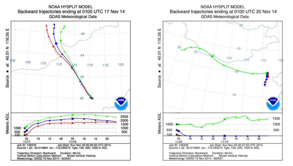
The result is fairly intuitive. On November 17, one important reason for the good air quality appears to be airflow from the northwest. The air masses that eventually reached 100 m, 500 m, and 1000 m above Beijing had actually descended from higher elevations. Since many pollution sources are located near the surface rather than high in the atmosphere, the source region suggested by this path was likely relatively clean. Looking at the latitude and longitude, this was essentially a northeasterly flow. Its height dropped sharply shortly before arrival, probably after encountering a local low-pressure area. About six hours before reaching Beijing, the air mass had just entered the Beijing–Tianjin–Hebei region. It is hard to say from this plot alone whether that low-pressure feature came from the urban heat-island effect, local terrain, or some other cause. But judging by the air quality that day, this air mass was probably one of the reasons conditions were better.

November 20 looks different. The high-altitude airflow also came from the northwest, and the distance it traveled in 48 hours suggests relatively strong winds aloft. But once the middle and lower layers are examined, the picture changes. Wind fields can vary greatly by altitude. The middle- and low-level airflows came from the southwest at lower altitude, and within the final six hours they showed an upward movement. That suggests Beijing may have been under the control of a high-pressure system that day, with a more stable atmosphere. Because the incoming air was low-level flow, it may have picked up pollutants from the southwest and transported them into Beijing. If other meteorological conditions were also favorable for accumulation, poor air quality that day would not be surprising.

This is the value of backward trajectory analysis: it can help explain the formation of a specific pollution event. Used together with source-apportionment methods, it allows researchers to sketch a more complete picture of where pollutants came from, how they moved, and where they went.

HYSPLIT is not limited to looking backward. It can also be used in forecast mode, so it is possible to estimate the future dispersion pathway of pollutants from a point source over the next few days. That can matter a great deal for real-time decision-making during emergency air-pollution incidents. The catch is resolution. Very high-precision data of this type seem to be available mainly for the United States. Global datasets are usually adequate for estimating airflow sources and transport paths at the urban-region scale, but for finer local analysis, one generally needs to collect more detailed data independently.

There is also an important limitation: this technique is not a magic key. It is a model-based prediction tool built on observational data. Roughly speaking, the underlying data divide the Earth into grid cells, place monitoring points every few degrees, and record variables such as elevation, wind speed, temperature, and air pressure. A dynamical model then connects and interpolates those grid values to estimate the path of the air mass being studied, finally reconstructing a likely main airflow route.

When the wind is strong, the results are often easier to interpret. When there is little wind, the model may reveal much less. It is common to see an air mass circling within a very small area, which may simply mean there was no meaningful transport at that time. Playing with the model can be interesting, but one piece of evidence is never enough. The more independent angles support the same explanation, the more reliable the conclusion becomes.

Still, it is worth trying. With only a basic grasp of geography, it is possible to get a rough idea of where the air over your city has come from and whether its path was likely clean or polluted. You may not be able to visit every corner of the world, but you can at least trace where the wind from those corners has traveled. Wind direction, after all, means the direction the wind blows from.